DL| U-Net 논문 리뷰 및 구현

09 Jun 2025 in Blog / DL on U-net, Biomedical image segmentation

U-Net 논문 리뷰를 통해 구조 및 biomedical image segmentation에서의 응용을 정리하고, PyTorch 기반 구현으로 세부 구조와 학습 방식을 분석

U-Net paper BoostCampAITECH

• Abstract
• Introduction
  • biomedical image
  • 이전 논문들
  • unet은 more elegant architecture
    • [9]의 main idea
  • one important modification in our architecture
    • data augmentataion
  • Network Architecture
    • contracting path
    • expansive path
• Training
  • 메모리 최적화
  • Loss function
  • good initialization of the weights in extremely important
  • Data Augmentataion
• Experiments
• Conclusion
• U-Net의 한계점
• U-Net 구현

• deep learning은 파라미터 수가 많고 네트워크가 깊어서 train data가 많이 필요
• biomedical의 특성상 데이터의 수가 많이 부족(전문가 라벨링 작업 및 개인 정보 때문에)
• cell segmentataion의 경우 같은 클래스가 인접해 있는 셀 사이 경계 구분이 필요한데 같은 클래스 지만 서로 다른 인스턴스로 구분이 필요함

→ 일반적인 semantic segmentation 작업에서는 불가능

Abstract

deep net-works requires many thousand annotated training samples

• data augmentataion
• architecture
  • contracting path: to capture context
  • expanding path: that enables precies localization

Introduction

biomedical image

classification task: output to an image is a single class label

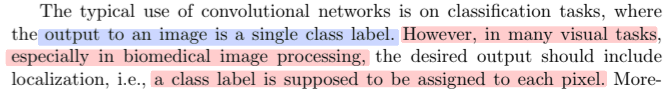
많은 visual tasks 중

biomedical image: 이미지 안에 여러개의 세포가 들어있기 때문에 픽셀별로 클래스를 분류해야하는 것이 필요(output should include localization(i.e. a class label is supposed to be assigned to each pixel.)

이전 논문들

이를 해결하기 위해서 여러 방식이 나오는데 unet 논문에서는 한 가지를 언급(EM segmentataion challenge at ISBI 2012에서 이겼던 ‘Deep neural networks segment neuronal membranes in electron microscopy images’)

sliding-window의 방식으로 학습시키고, 각 픽셀 주위의 지역 영역(패치)을 입력으로 제공함으로써 각 픽셀의 클래스 레이블을 예측하게 함

1. this network can localize
2. the training data in terms of patches is much larger than the number of training images

해당 논문의 문제점

• quite slow
  • the network must be run separately for each patch, and there is a lot of redundancy due to overlapping patches.
• trade-off between localization accuracy and the use of context
  • larger patches require more max-pooling layers that reduce the localization accuracy
  • while small patches allow the network to see only little context

최근 접근법들에서는 여러 계층의 특징을 반영하는 분류기 출력을 제안, 이를 통해서 good localization and the use of context are possible at the same time을 할 수 있음

unet은 more elegant architecture

‘Fully Convolutional Networks for Semantic Segmentation’(FCN)[9]를 수정하고 확장하여 적은 이미지, 정확한 segmentation이 가능하도록 함

[9]의 main idea

1. usual contracting network를 successive layers로 보완하며 pooling layer는 upsampling layer로 대체 → increase the resolution of the output
2. order to localize를 하기 위해서 contracting path의 high resolution fatures를 upsampled output과 combined → A successive convolution layer can then learn to assemble a more precise output based on this infomration

one important modification in our architecture

• upsampling part에 large number fo feature channels를 둠
  • which allow the network to propagate context information to higher resolution layers.
  • 그 결과, expansive path는 contracting path와 대칭을 이루면서 U자형 구조로 형성
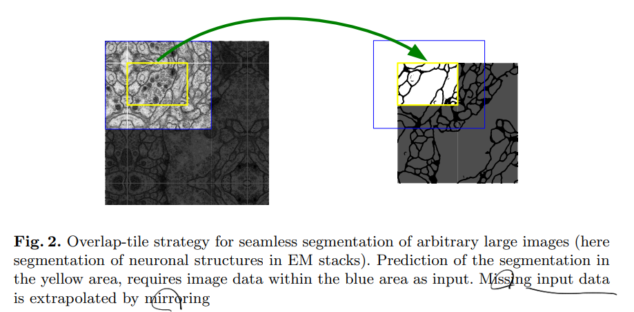
• overlap-tile strategy
  • fully connected layers는 포함되지 않음
  • 각 convolution의 유효한 부분만을 사용함 즉, segmentation map에는 입력 이미지에서 전체 context가 확보된 픽셀만 포함

  • 임의 크기의 이미지를 매끄럽게 분할할 수 있게 하며 이미지 경계 픽셀을 예측하기 위해서 부족한 context는 Extrapolation 기법을 적용 → 네트워크를 대형 이미지에 적용하는데 중요하고 그렇지 않으면 해상도가 GPU 메모리에 의해 제한됨

    

data augmentataion

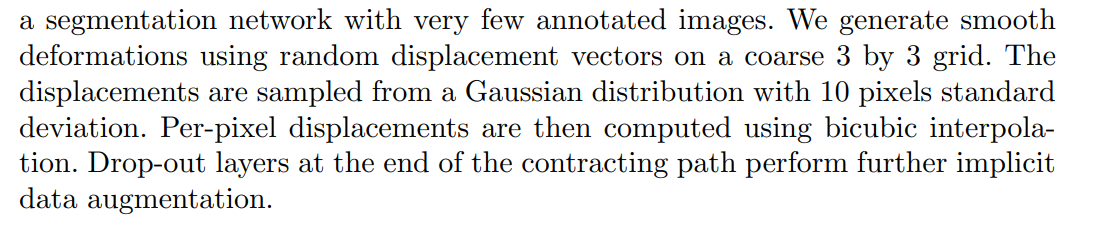
데이터의 양이 적기 때문에 데이터 증강을 통해 Noise에 강건하도록 학습하였고 Rotataion, Shift, Elastic destortion 등을 사용

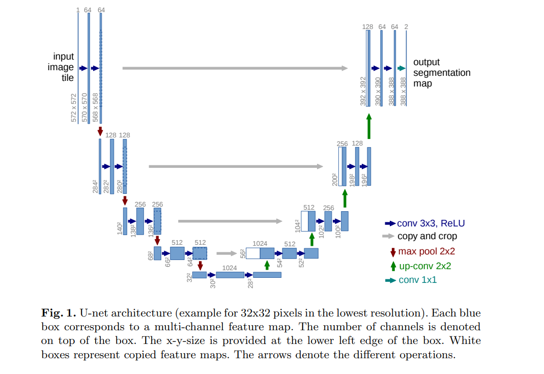
Network Architecture

contracting path

Downsampling 과정을 반복하여 feature map을 만듦, downsampling을 할 때 마다 채널의 수를 2배 증가시키면서 진행

1. 3x3 convolution layer + ReLu
2. 3x3 convolution layer + ReLu
3. 2x2 Max-polling Layer(Stride 2)

• 1, 2 이후에 + BatchNorm(No Padding, Stride 1)를 구현할 때 대체로 적용시킴

expansive path

Upsampling과정을 반복하면서 feature map을 생성

1. 2x2 Deconvolution layer(Stride 2): Pytorch의 ConvTranspose2d
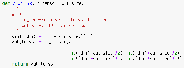
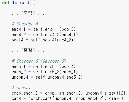
2. Contracting path에서 동일 level의 특징맵을 추출하고 크기를 맞추기 위해 cropping, 이전 layer에서 생성된 feature map과 concat: 동일한 Level에서 contracting path와 크기가 다른 이유는 여러 번의 패딩이 없는 3x3 convolution layer를 지나면서 feature map의 크기가 줄어들기 때문
3. 3×3 Convolution Layer + ReLu + BatchNorm (No Padding, Stride 1)
4. 3×3 Convolution Layer + ReLu + BatchNorm (No Padding, Stride 1)

final layer에서는 1x1 convolution을 사용하여 각 64차원 특징 벡터를 원하는 클래스 수로 매핑, 네트워크는 총 23개의 convolution layer로 구성됨

Training

메모리 최적화

• unpadded convolution으로 인해서 output image는 일정한 경계 폭만큼 input보다 더 작음 → overhead 최소화, GPU 메모리 최대 활용
  • 큰 배치 크기보다 큰 input tiles를 선호하여 batch_size를 1로 함
  • 높은 momentum(0.99)을 사용

  → 이전 학습 샘플이 현재 최적화 단계의 업데이트에 영향을 미치도록 함

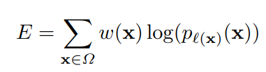
Loss function

energy function: final feature map에 픽셀 단위로 soft-max를 하고 cross entropy loss function을 적용하는 식

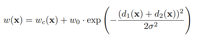
x(feature map에 있는 각 픽셀)로 각 픽셀에서 계산한 것을 다 더한 것, w(x)는 weight map이라고 픽셀 별로 가중치를 부과하는 역할

weight map: to balance the class frequencies: 각 세포 사이의 경계를 잘 포착해야하며 학습 데이터에서 각 픽셀마다 클래스 분포가 다른 점을 고려하여 weight map을 구해 학습에 반영

• $w_c(x)$: class별 빈도에 따른 가중치
• $d_1$: 가장 인접한 cell과의 거리
• $d_2$: 두번째로 인접한 cell과의 거리
• $w_0 = 10$, $\sigma = 5$

good initialization of the weights in extremely important

노드의 개수가 N이라면 root(2/N)의 표준편차를 가진 가우시안 분포를 이용해서 가중치를 초기화

E.g. for a 3x3 convolution and 64 feature channles in the previous layer N= 9 * 64 = 576

Data Augmentataion

데이터 수가 적을 때 필수적임, microsopical images(현미경 촬영 이미지)는 shift and rotation invariance as well as robustness to deformations and gray value variations.

shift, rotation 외에 random-elastic deformation이라는 기법을 사용하여 증강을 구한하였고 random-elastic deformation은 작은 데이터를 가지고 segmentation network를 학습시킬 때 key concept로 보인다고 함

구현순서

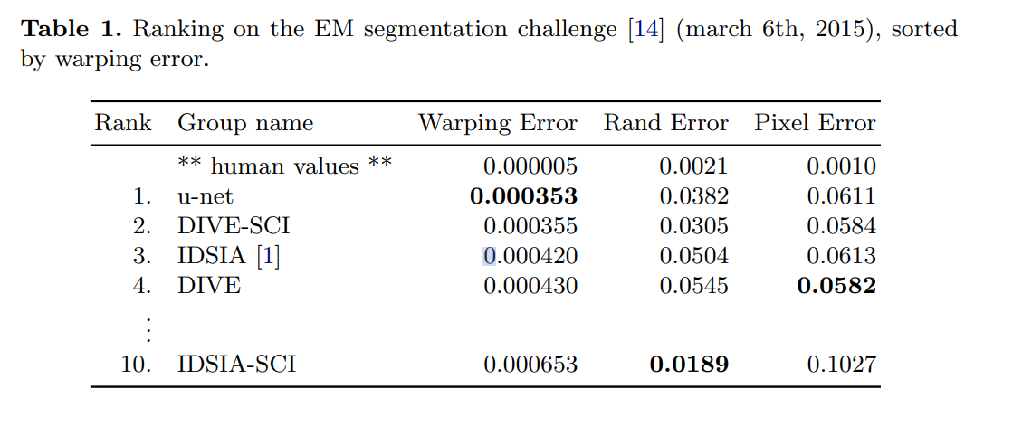
Experiments

EM Segmentation challenge

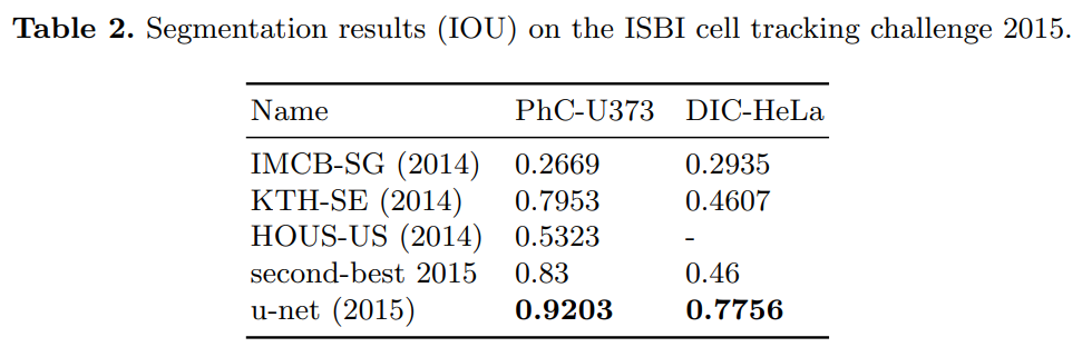
ISBI cell tracking challenge

Conclusion

biomdical segmentataion applications에서 좋은 성능을 보임, 합리적인 학습시간을 가졌으며 U-Net의 구조가 다양한 task에 사용이 될 것

U-Net의 한계점

• U-Net은 기본적으로 깊이가 4로 고정이 되어 있어 데이터셋마다 최고의 성능을 보장하지 못하며 최적 깊이 탐색 비용이 높음
• 단순한 Skip Connection으로 동일한 깊이를 가지는 Encoder Decoder만 연결되는 제한적인 구조

U-Net 구현

class UNet(nn.Module):
    def __init__(self, num_classes=len(CLASSES)):
        super(UNet, self).__init__()
        def CBR2d(in_channels, out_channels, kernel_size=3, stride=1, padding=1, bias=True):
            layers = []
            layers += [nn.Conv2d(in_channels=in_channels, out_channels=out_channels,
                                 kernel_size=kernel_size, stride=stride, padding=padding, bias=bias)]
            layers += [nn.BatchNorm2d(num_features=out_channels)]
            layers += [nn.ReLU()]

            cbr = nn.Sequential(*layers)
            return cbr

        # Contracting path
        # Encoder 1: 구현체에 따라서 padding을 1로 주어 크기 고정하기도 함
        self.enc1_1 = CBR2d(in_channels=3, out_channels=64, kernel_size=3, stride=1, padding=1, bias=True)
        self.enc1_2 = CBR2d(in_channels=64, out_channels=64, kernel_size=3, stride=1, padding=1, bias=True)
        self.pool1 = nn.MaxPool2d(kernel_size=2)
				
        # Encoder 2
        self.enc2_1 = CBR2d(in_channels=64, out_channels=128, kernel_size=3, stride=1, padding=1, bias=True)
        self.enc2_2 = CBR2d(in_channels=128, out_channels=128, kernel_size=3, stride=1, padding=1, bias=True)
        self.pool2 = nn.MaxPool2d(kernel_size=2)
        
        # Encoder 3
        self.enc3_1 = CBR2d(in_channels=128, out_channels=256, kernel_size=3, stride=1, padding=1, bias=True)
        self.enc3_2 = CBR2d(in_channels=256, out_channels=256, kernel_size=3, stride=1, padding=1, bias=True)
        self.pool3 = nn.MaxPool2d(kernel_size=2)
        
        # Encoder 4
        self.enc4_1 = CBR2d(in_channels=256, out_channels=512, kernel_size=3, stride=1, padding=1, bias=True)
        self.enc4_2 = CBR2d(in_channels=512, out_channels=512, kernel_size=3, stride=1, padding=1, bias=True)
        self.pool4 = nn.MaxPool2d(kernel_size=2)
				
        # Encoder 5 || Decoder 5
        self.enc5_1 = CBR2d(in_channels=512, out_channels=1024, kernel_size=3, stride=1, padding=1, bias=True)
        self.enc5_2 = CBR2d(in_channels=1024, out_channels=1024, kernel_size=3, stride=1, padding=1, bias=True)
        self.unpool4 = nn.ConvTranspose2d(in_channels=1024, out_channels=512, kernel_size=2, stride=2, padding=0, bias=True)

        self.dec4_2 = CBR2d(in_channels=1024, out_channels=512, kernel_size=3, stride=1, padding=1, bias=True)
        self.dec4_1 = CBR2d(in_channels=512, out_channels=512, kernel_size=3, stride=1, padding=1, bias=True)

        self.unpool3 = nn.ConvTranspose2d(in_channels=512, out_channels=256, kernel_size=2, stride=2, padding=0, bias=True)

        self.dec3_2 = CBR2d(in_channels=512, out_channels=256, kernel_size=3, stride=1, padding=1, bias=True)
        self.dec3_1 = CBR2d(in_channels=256, out_channels=256, kernel_size=3, stride=1, padding=1, bias=True)

        self.unpool2 = nn.ConvTranspose2d(in_channels=256, out_channels=128, kernel_size=2, stride=2, padding=0, bias=True)

        self.dec2_2 = CBR2d(in_channels=256, out_channels=128, kernel_size=3, stride=1, padding=1, bias=True)
        self.dec2_1 = CBR2d(in_channels=128, out_channels=64, kernel_size=3, stride=1, padding=1, bias=True)

        self.unpool1 = nn.ConvTranspose2d(in_channels=64, out_channels=64, kernel_size=2, stride=2, padding=0, bias=True)

        self.dec1_2 = CBR2d(in_channels=128, out_channels=64, kernel_size=3, stride=1, padding=1, bias=True)
        self.dec1_1 = CBR2d(in_channels=64, out_channels=64, kernel_size=3, stride=1, padding=1, bias=True)
        self.score_fr = nn.Conv2d(in_channels=64, out_channels=num_classes, kernel_size=1, stride=1, padding=0, bias=True) # Output Segmentation map

    def forward(self, x):
        enc1_1 = self.enc1_1(x)
        enc1_2 = self.enc1_2(enc1_1)
        pool1 = self.pool1(enc1_2)

        enc2_1 = self.enc2_1(pool1)
        enc2_2 = self.enc2_2(enc2_1)
        pool2 = self.pool2(enc2_2)

        enc3_1 = self.enc3_1(pool2)
        enc3_2 = self.enc3_2(enc3_1)
        pool3 = self.pool3(enc3_2)

        enc4_1 = self.enc4_1(pool3)
        enc4_2 = self.enc4_2(enc4_1)
        pool4 = self.pool4(enc4_2)

        enc5_1 = self.enc5_1(pool4)
        enc5_2 = self.enc5_2(enc5_1)
			
        unpool4 = self.unpool4(enc5_2)
        cat4 = torch.cat((unpool4, enc4_2), dim=1)
        dec4_2 = self.dec4_2(cat4)
        dec4_1 = self.dec4_1(dec4_2)

        unpool3 = self.unpool3(dec4_1)
        cat3 = torch.cat((unpool3, enc3_2), dim=1)
        dec3_2 = self.dec3_2(cat3)
        dec3_1 = self.dec3_1(dec3_2)

        unpool2 = self.unpool2(dec3_1)
        cat2 = torch.cat((unpool2, enc2_2), dim=1)
        dec2_2 = self.dec2_2(cat2)
        dec2_1 = self.dec2_1(dec2_2)

        unpool1 = self.unpool1(dec2_1)
        cat1 = torch.cat((unpool1, enc1_2), dim=1)
        dec1_2 = self.dec1_2(cat1)
        dec1_1 = self.dec1_1(dec1_2)

        output = self.score_fr(dec1_1)
        return output

padding=’same’을 이용하여 convolution 이후에도 feature map의 크기가 유지되도록 하여 cropping 과정을 생략, 원래는 밑의 코드를 사용함